[Geometry optimization and vibrational analysis]
The geometry optimization and vibrational analysis of a molecule using CONFLEX are explained.
[Execution of geometry optimization and vibrational analysis]
This section explains how to perform the geometry optimization and vibrational analysis using cyclohexane as an example. First, prepare a structure file of cyclohexane molecule in MDL-MOL format as Cyclohexane.mol. The Cyclohexane.mol is located in the Sample_Files folder where CONFLEX is installed (Sample_Files\CONFLEX\optimization_and_search\Cyclohexane.mol).
Cyclohexane.mol file

- A1: The number of atoms (up to 999)
- A2: The number of bonds (up to 999)
- A3: Currently not use
- A4: Currently not use
- A5: Existence of optically active center (0: not have, 1: have) : Currently not use
- B1: Cartesian coordinates and symbols of atoms
- B2: Physical property list of atoms (Isotopes, charge, stereocenter, and so on set. In general, only charge and stereocenter are required.)
- C1: Information on bonds between atoms (Information on adjacent bonds when atoms are the center is indicated. The bonding state, three-dimensional state, bonding topology and the like are indicated. Usually only information on bonds between adjacent atoms, bonding state and three-dimensional state are required.
- D1: This indicates that atomic conformation has been completed and is necessary information.
[Execution from Interface]
Open the Cyclohexane.mol file using CONFLEX Interface.

Select [CONFLEX] from the Calculation menu, and then click in the calculation setting dialog that appears. The calculations of molecular geometry optimization and normal mode analysis will be performed.

[Execution from command line]
Store the Cyclohexane.mol in a folder, and execute the following command to start the calculation.
C:\CONFLEX\bin\conflex-10a.exe -par C:\CONFLEX\par Cyclohexaneenter
The command above is for Windows OS. For other OS, please refer to [How to execute CONFLEX].
If there is no ini file in the folder, the calculation of molecular geometry optimization and normal mode analysis will be performed with default settings. In this case, the calculation is the same as if you had prepared the Cyclohexane.ini file that describes [MMFF94S OPT=NEWTON OPTBY=ENERGY] in the folder.
[Output files]
After the calculation is complete, three files will be output, as shown below.
Cyclohexane-F.mol
The optimized structure is output to this file in MDL-MOL format. The file format depends on the input structure file.
Cyclohexane.mol
CONFLEX 20090414283D 1   1.00000    -3.56094     0
D3D ,E =   -3.561, G = 6.035E-11, M(0)      MMFF94S(2010-12-04HG)
 18 18  0     0               999 V2000
   -1.2627    0.7290    0.2258 C   0  0  0  0  0
    0.0000    1.4580   -0.2258 C   0  0  0  0  0
   -1.2627   -0.7290   -0.2258 C   0  0  0  0  0
   -2.1462    1.2391   -0.1742 H   0  0  0  0  0
   -1.3365    0.7716    1.3195 H   0  0  0  0  0
   -0.0000    2.4782    0.1742 H   0  0  0  0  0
    0.0000    1.5433   -1.3195 H   0  0  0  0  0
    0.0000   -1.4580    0.2258 C   0  0  0  0  0
   -2.1462   -1.2391    0.1742 H   0  0  0  0  0
   -1.3365   -0.7716   -1.3195 H   0  0  0  0  0
    0.0000   -2.4782   -0.1742 H   0  0  0  0  0
    0.0000   -1.5433    1.3195 H   0  0  0  0  0
    1.2627   -0.7290   -0.2258 C   0  0  0  0  0
    2.1462   -1.2391    0.1742 H   0  0  0  0  0
    1.3365   -0.7716   -1.3195 H   0  0  0  0  0
    1.2627    0.7290    0.2258 C   0  0  0  0  0
    1.3365    0.7716    1.3195 H   0  0  0  0  0
    2.1462    1.2391   -0.1742 H   0  0  0  0  0
  2  1  1  0     0
  3  1  1  0     0
  1  4  1  0     0
  1  5  1  0     0
  2  6  1  0     0
  2  7  1  0     0
  2 16  1  0     0
  3  8  1  0     0
  3  9  1  0     0
  3 10  1  0     0
 11  8  1  0     0
 12  8  1  0     0
 13  8  1  0     0
 14 13  1  0     0
 13 15  1  0     0
 16 13  1  0     0
 16 17  1  0     0
 16 18  1  0     0
M  END
Cyclohexane.bsf
The atomic coordinates, energy value, etc of the optimized structure are output to this file.
999.9 6 0 6  0 1  0  010.00  1.00E-06  1.00E-06   0   0 25.000010001100000000000
Cyclohexane: Cyclohexane.mol
D3D ,E =   -3.561, G = 6.035E-11, M(0)      MMFF94S(2010-12-04HG)
18 18
 0.00000   0.00000   0.00000   0.00000   0.00000   0.00000   0.00000   0.00000
 0.00000   0.00000   0.00000   0.00000   0.00000   0.00000   0.00000   0.00000
 0.00000   0.00000
-1.262673724   0.729005014   0.225782342  6  0 12   2   3   4   5   0   0   1
 0.000000000   1.458010029  -0.225782342  6  0 12   1   6   7  16   0   0   2
-1.262673724  -0.729005014  -0.225782342  6  0 12   1   8   9  10   0   0   3
-2.146189104   1.239102857  -0.174187977  1  0  1   1   0   0   0   0   0   4
-1.336507200   0.771632792   1.319462875  1  0  1   1   0   0   0   0   0   5
-0.000000000   2.478205714   0.174187977  1  0  1   2   0   0   0   0   0   6
 0.000000000   1.543265583  -1.319462875  1  0  1   2   0   0   0   0   0   7
 0.000000000  -1.458010029   0.225782342  6  0 12   3  11  12  13   0   0   8
-2.146189104  -1.239102857   0.174187977  1  0  1   3   0   0   0   0   0   9
-1.336507200  -0.771632792  -1.319462875  1  0  1   3   0   0   0   0   0  10
 0.000000000  -2.478205714  -0.174187977  1  0  1   8   0   0   0   0   0  11
 0.000000000  -1.543265583   1.319462875  1  0  1   8   0   0   0   0   0  12
 1.262673724  -0.729005014  -0.225782342  6  0 12   8  14  15  16   0   0  13
 2.146189104  -1.239102857   0.174187977  1  0  1  13   0   0   0   0   0  14
 1.336507200  -0.771632792  -1.319462875  1  0  1  13   0   0   0   0   0  15
 1.262673724   0.729005014   0.225782342  6  0 12   2  13  17  18   0   0  16
 1.336507200   0.771632792   1.319462875  1  0  1  16   0   0   0   0   0  17
 2.146189104   1.239102857  -0.174187977  1  0  1  16   0   0   0   0   0  18
Cyclohexane.bso
This file contains the force field parameters used in the calculation, energies of each interaction as well as thermodynamic quantities, frequencies, and vibrational modes obtained from the normal mode analysis, etc.

- (A-1): Name of force field used in the calculation
- (A-2): Information about atom types assigned to atoms composing of input molecule
- (A-3): Function of bond stretching interaction and its parameters in the force field
- Functions of other interactions and their parameters are shown after the section A-3.

- (A-4): Initial coordinates and serial numbers of atoms
- (A-5): Atom types assigned to atoms
- (A-6): Bond information
- (A-7): Energy gradients with respect to input structure

- (A-8): Inertia moment and dipole moment of input structure
- (A-9): Steric energies of each interaction function term for input structure

- (A-10):Process of geometry optimization by Newton-Raphson method
- (A-11):Geometry optimization has converged.
- (A-12):Final eigenvalues. The number of zero eigenvalues is 5 for linear molecules and 6 for other molecules.

- (A-13): Structural parameters and energies of each interaction in the input molecule.

- (A-14): The partition function amount relating to internal energy, enthalpy, entropy, Gibbs free energy and constant pressure heated capacity are calculated taking into account the details of the thermodynamic functions, the temperature designated and the symmetry of the optimized structure.
- (A-15): The number of imaginary, zero, and real frequencies. You should check that the optimized structure has 6 zero-frequencies and doesn't have any imaginary frequencies.

- (A-16): Frequencies and vibrational modes. The vibrational modes are shown as displacement vectors in Cartesian coordinate system. By using a keyword, these vectors can also be shown in an internal coordinate system.
[Visualization of calculation results]
[If you executed the calculation using Interface]
After submitting a job, Job Manager is appeared at bottom of CONFLEX Interface. Job Manager shows a state of the job.

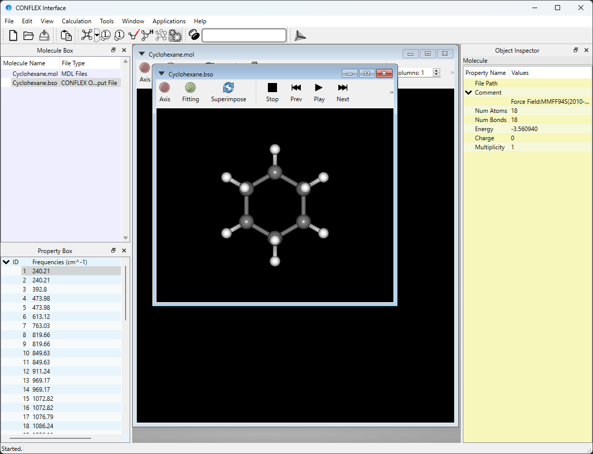
Check that the state of the job is “Finished”, and then double-click the row of the job (indicated by red frame).
Cyclohexane.bso will open automatically, and the optimized structure will be displayed. The Cyclohexane.bso file is located in the folder containing the input files.

Select [Vibration] from the View menu. Displacement vectors of atoms due to normal vibrations will be displayed.

* You can change the magnitude of the arrows by changing the value of [5.0 x] in the toolbar.
[If you executed the calculation using command line]
Open either the Cyclohexane-F.mol or Cyclohexane.bso file using the CONFLEX Interface. The optimized structure will be displayed. These files are located in the folder containing the input files.
If you open Cyclohexane.bso, you can view displacement vectors of atoms due to normal vibrations by selecting [Vibration] from the View menu.
* You can change the magnitude of the arrows by changing the value of [5.0 x] in the toolbar.
[Calculation including solvent effects]
Introduce solvent effects using GB/SA model
When compounds are synthesized and their structures and physical properties are measured in chemical experiments, these experiments are almost always conducted in solution. Therefore, when analyzing experimentally observed phenomena using molecular calculations, it is essential to consider the solution phase. However, common molecular force fields are typically constructed under the assumption that the compound is in the gas phase, and solvent effects are generally not taken into account. While a more accurate approach would involve including a large number of solvent molecules around the solute, doing so significantly increases the number of degrees of freedom, which in turn leads to a substantial increase in computation time.
To address this issue, research on incorporating solvent effects using a continuous dielectric model has long been conducted in the field of molecular calculations. When using CONFLEX, the GB/SA model, one of the most widely used the continuous dielectric model in molecular dynamics simulations, is employed. This allows for the computation of geometry optimization, vibrational analysis, and solvation free energy, all of which include solvent effects. In the current version, the MMFF94s force field is used, and octanol is considered as the solvent.
What is GB/SA model ?
The GB/SA model calculates the electrostatic contribution of the solvent using the Generalized Born (GB) equation, while the non-electrostatic contribution is estimated based on the solvent-accessible surface area (SA). The amount of increase in energy caused by the solvent is expressed as

The electrostatic term becomes

using the GB equation and the non-electrostatic term is calculated as

Here, the qi is a charge of atom i, the rij is distance between atoms i and j, the αij and Dij are values obtained by effective Born radius, the σkis a surface tension coefficient, and the SAk is a solvent-accessible surface area of atom k.
In CONFLEX9 and later, [SA=IGNORE] keyword has been added to ignore the non-electrostatic term in the calculation. If a geometry optimization with solvent effects is not converge, please add this keyword to the calculation setting.
Calculation using GB/SA model
We use a zwitterionic glycine dimer.

Structure data of the zwitterionic glycine dimer (gly2.mol)
gly2.mol


 17 16  0  0  0  0  0  0  0  0999 V2000
   -1.2219    0.9765   -2.1504 N   0  3  0  0  0  0  0  0  0  0  0  0
    0.2781    0.9765   -2.1504 C   0  0  0  0  0  0  0  0  0  0  0  0
    0.6496    2.0256   -2.1504 H   0  0  0  0  0  0  0  0  0  0  0  0
    0.7803    0.2658   -0.9176 C   0  0  0  0  0  0  0  0  0  0  0  0
    1.9679    0.1552   -0.7258 O   0  0  0  0  0  0  0  0  0  0  0  0
   -0.1098   -0.2537   -0.0165 N   0  0  0  0  0  0  0  0  0  0  0  0
    0.3728   -0.9366    1.1681 C   0  0  0  0  0  0  0  0  0  0  0  0
    0.9911   -0.2372    1.7741 H   0  0  0  0  0  0  0  0  0  0  0  0
   -0.8018   -1.4089    1.9892 C   0  0  0  0  0  0  0  0  0  0  0  0
   -0.6088   -2.0256    3.0592 O   0  0  0  0  0  0  0  0  0  0  0  0
   -1.9679   -1.1835    1.5993 O   0  5  0  0  0  0  0  0  0  0  0  0
   -1.5708    0.4839   -3.0034 H   0  0  0  0  0  0  0  0  0  0  0  0
   -1.5698    0.4832   -1.2973 H   0  0  0  0  0  0  0  0  0  0  0  0
   -1.5701    1.9618   -2.1504 H   0  0  0  0  0  0  0  0  0  0  0  0
    0.6489    0.4518   -3.0592 H   0  0  0  0  0  0  0  0  0  0  0  0
   -1.1047   -0.1611   -0.1772 H   0  0  0  0  0  0  0  0  0  0  0  0
    0.9910   -1.8114    0.8658 H   0  0  0  0  0  0  0  0  0  0  0  0
  1  2  1  0
  1 12  1  0
  1 13  1  0
  1 14  1  0
  2  3  1  0
  2  4  1  0
  2 15  1  0
  4  5  2  0
  4  6  1  0
  6  7  1  0
  6 16  1  0
  7  8  1  0
  7  9  1  0
  7 17  1  0
  9 10  2  0
  9 11  1  0
M  END
[Execution from Interface]
Open the gly2.mol file using CONFLEX Interface.

Select [CONFLEX] from the Calculation menu, and then click in the calculation setting dialog that appears.

Next, in [Force Field] dialog of the detailed settings dialog, select [GBSA] from the pull-down menu of [Solvent Effect].

After completing the calculation settings, click to start the calculation.
[Execution from command line]
The calculation settings are defined by specifying keywords in the gly2.ini file.
gly2.ini file
MMFF94S GBSA
[GBSA] means to execute the calculation including solvent effects using GB/SA model.
[MMFF94S] means to use the MMFF94s force field.
Store the two files of gly2.mol and gly2.ini in to a single folder, and execute the following command to start the caluclation.
C:\CONFLEX\bin\conflex-10a.exe -par C:\CONFLEX\par gly2enter
The command above is for Windows OS. For other OS, please refer to [How to execute CONFLEX].
Calculation results
The optimized structure is shown below. For how to visualize this, please refer to [Visualization of calculation results].

[Geometry optimization with constraints]
In the geometry optimization, all degrees of freedom of the atoms are relaxed. However, the geometry optimization with constraints, which fix certain parts of the structure, may be necessary in some cases. This is useful, for example, when you want to optimize only the unknown parts of a structure that are partially known, or when you wish to optimize while keeping certain structural parameters fixed. In CONFLEX, the geometry optimization with the constraints can be performed by three methods described below.
- Constraint by harmonic potential
- Constraint by molecular object method
- Constraint by freezing atomic coordinates
These methods can apply to a conformational search.
* Constraint by harmonic potential
It is possible to inpose restrictions on the geometry optimization by adding pseudo potentials to structural parameters such as interatomic distance, bond angle, dihedral angle, and so on. Keywords for adding the pseudo potentials to each structural parameter are as follows:
| Structural parameter | Keyword | Explanation |
|---|---|---|
| Bond length | PSEUDO_BOND=(I,J,STD,FK) | The harmonic potential with the standard length STD (Å) and the force constant FK (kcal・mol-1・Å-2) is applied to the atomic pair of I and J. |
| PSEUDO_HALF=(I,J,STD,FK) | The half-harmonic potential with the standard length |STD| (Å) and the force constant FK (kcal・mol-1・Å-2) is applied to the atomic pair of I and J. In the case of STD>0, the energy increases as the distance between I-J becomes longer than STD. On the other hand, in case of STD<0, the energy increases as the distance between I-J becomes shorter than STD. | |
| Valence angle | PSEUDO_ANGL=(I,J,K,STD,FK) | The harmonic potential with the standard angle STD (°) and the force constant FK (kcal・mol-1・rad-2) is applied to the valence angle of I-J-K. |
| Dihedral angle | PSEUDO_TORS=(I,J,K,L,STD,FK) | The harmonic potential with the standard angle STD (°) and the force constant FK (kcal・mol-1・rad-2) is applied to the dihedral angle of I-J-K-L. |
Example calculation
This section explains a geometry optimization of n-butane with trans conformation using the pseudo potential for maintaining C-C-C-C dihedral angle to around 150.0.
Three dimensional structure of n-butane

Structure data of n-butane (n-butane.mol)
n-butane.mol


 14 13  0  0  0  0  0  0  0  0999 V2000
   -1.1802   -1.5102    0.0000 C   0  0  0  0  0  0  0  0  0  0  0  0
    0.1388   -0.7487    0.0000 C   0  0  0  0  0  0  0  0  0  0  0  0
   -0.1388    0.7487    0.0000 C   0  0  0  0  0  0  0  0  0  0  0  0
    1.1802    1.5102    0.0000 C   0  0  0  0  0  0  0  0  0  0  0  0
   -0.9774   -2.6046    0.0000 H   0  0  0  0  0  0  0  0  0  0  0  0
   -1.7631   -1.2415    0.9093 H   0  0  0  0  0  0  0  0  0  0  0  0
   -1.7637   -1.2413   -0.9088 H   0  0  0  0  0  0  0  0  0  0  0  0
    0.7217   -1.0175   -0.9093 H   0  0  0  0  0  0  0  0  0  0  0  0
    0.7223   -1.0177    0.9088 H   0  0  0  0  0  0  0  0  0  0  0  0
   -0.7217    1.0175    0.9093 H   0  0  0  0  0  0  0  0  0  0  0  0
   -0.7223    1.0177   -0.9088 H   0  0  0  0  0  0  0  0  0  0  0  0
    0.9774    2.6046    0.0000 H   0  0  0  0  0  0  0  0  0  0  0  0
    1.7631    1.2415   -0.9093 H   0  0  0  0  0  0  0  0  0  0  0  0
    1.7637    1.2412    0.9088 H   0  0  0  0  0  0  0  0  0  0  0  0
  1  2  1  0
  1  5  1  0
  1  6  1  0
  1  7  1  0
  2  3  1  0
  2  8  1  0
  2  9  1  0
  3  4  1  0
  3 10  1  0
  3 11  1  0
  4 12  1  0
  4 13  1  0
  4 14  1  0
M  END
[Execution from Interface]
Open the n-butane.mol file using CONFLEX Interface.

Select [CONFLEX] from the Calculation menu, and then click in the calculation setting dialog that appears. Next, click at the bottom Next, click at the bottom right of the detailed settings dialog..

Add [PSEUDO_TORS=(1,2,3,4,150.0,100.0)] to the dialog that appears. By this keyword, the harmonic potential with the standard angle 150 (°) and the force constant 100.0 (kcal・mol-1・rad-2) adds to the dihedral angle of C-C-C-C. After completing the calculation settings, click to start the calculation.

[Execution from command line]
The calculation settings are defined by specifying keywords in the n-butane.ini file.
n-butane.ini file
MMFF94S
PSEUDO_TORS=(1,2,3,4,150.0,100.0)
[MMFF94S] means to use MMFF94s force field.
[PSEUDO_TORS=(1,2,3,4,150.0,100.0)] means that the harmonic potential with the standard angle 150 (°) and the force constant 100.0 (kcal・mol-1・rad-2) adds to the dihedral angle of C-C-C-C.
Store the two files of n-butane.mol and n-butane.ini in a single folder, and execute the following command to start the calculation.
C:\CONFLEX\bin\conflex-10a.exe -par C:\CONFLEX\par n-butaneenter
The command above is for Windows OS. For other OS, please refer to [How to execute CONFLEX].
Calculation results
The larger the force constant value, the closer the dihedral angle of the optimized structure will be to the STD value. Table 1 shows the dihedral angles of structures optimized using different force constant settings.
Table 1: Force constant and C-C-C-C dihedral angle of the optimized structure
| Force constant (kcal・mol-1・rad-2) | Dihedral angle (°) |
|---|---|
| 10 | 168.6 |
| 100 | 153.4 |
| 1000 | 150.3 |
* Constraint by molecular object method
In the case of a system consists of more than one molecule, CONFLEX can optimize the specified molecules while kepping the others fixed. In this calculation, it is necessary to set both “OPT=GROUP” and “MOL_GROUP=(I,N)” keywords. Here, N and I in MOL_GROUP keyword are a group number and atom number for the molecule to be optimized, respectively.
Example calculation
We optimize only water molecule in the system consists of α-D-glucose and water.

Structure data (aDglucose_H2O.mol)
aDglucose_H2O.mol


 27 26  0  0  0               999 V2000
   -0.5024    2.4148    0.6016 O   0  0  0  0  0  0  0  0  0  0  0  0
   -0.8520   -1.0932   -0.5731 O   0  0  0  0  0  0  0  0  0  0  0  0
    0.4519   -1.5744   -0.2774 C   0  0  0  0  0  0  0  0  0  0  0  0
   -0.2020    1.2411   -0.1553 C   0  0  0  0  0  0  0  0  0  0  0  0
   -1.1949    0.1125    0.1452 C   0  0  0  0  0  0  0  0  0  0  0  0
    2.1431    1.8092   -0.2200 O   0  0  0  0  0  0  0  0  0  0  0  0
    0.5330   -1.9764    1.0847 O   0  0  0  0  0  0  0  0  0  0  0  0
    2.8319   -0.9820   -0.1321 O   0  0  0  0  0  0  0  0  0  0  0  0
   -2.6186    0.5024   -0.2701 C   0  0  0  0  0  0  0  0  0  0  0  0
    1.5391   -0.5233   -0.5592 C   0  0  0  0  0  0  0  0  0  0  0  0
    1.2184    0.7799    0.1723 C   0  0  0  0  0  0  0  0  0  0  0  0
   -3.5094   -0.5881   -0.0183 O   0  0  0  0  0  0  0  0  0  0  0  0
    0.2794    2.9953    0.4978 H   0  0  0  0  0  0  0  0  0  0  0  0
    0.6445   -2.4621   -0.8896 H   0  0  0  0  0  0  0  0  0  0  0  0
   -0.2535    1.5201   -1.2154 H   0  0  0  0  0  0  0  0  0  0  0  0
   -1.2141   -0.1177    1.2184 H   0  0  0  0  0  0  0  0  0  0  0  0
    3.0267    1.3889   -0.1951 H   0  0  0  0  0  0  0  0  0  0  0  0
   -0.0183   -2.7768    1.1469 H   0  0  0  0  0  0  0  0  0  0  0  0
    2.6839   -1.4193    0.7318 H   0  0  0  0  0  0  0  0  0  0  0  0
   -2.6702    0.7196   -1.3421 H   0  0  0  0  0  0  0  0  0  0  0  0
   -2.9791    1.3731    0.2851 H   0  0  0  0  0  0  0  0  0  0  0  0
    1.6027   -0.3262   -1.6358 H   0  0  0  0  0  0  0  0  0  0  0  0
    1.3472    0.6668    1.2558 H   0  0  0  0  0  0  0  0  0  0  0  0
   -3.0727   -1.3725   -0.4004 H   0  0  0  0  0  0  0  0  0  0  0  0
   -0.3106    0.8234   -2.7522 O   0  0  0  0  0  0  0  0  0  0  0  0
   -0.3290    0.0085   -2.2451 H   0  0  0  0  0  0  0  0  0  0  0  0
   -0.9697    0.7822   -3.4490 H   0  0  0  0  0  0  0  0  0  0  0  0
  1  4  1  0  0  0  0
  1 13  1  0  0  0  0
  2  3  1  0  0  0  0
  2  5  1  0  0  0  0
  3  7  1  0  0  0  0
  3 10  1  0  0  0  0
  3 14  1  0  0  0  0
  4  5  1  0  0  0  0
  4 11  1  0  0  0  0
  4 15  1  0  0  0  0
  5  9  1  0  0  0  0
  5 16  1  0  0  0  0
  6 11  1  0  0  0  0
  6 17  1  0  0  0  0
  7 18  1  0  0  0  0
  8 10  1  0  0  0  0
  8 19  1  0  0  0  0
  9 12  1  0  0  0  0
  9 20  1  0  0  0  0
  9 21  1  0  0  0  0
 10 11  1  0  0  0  0
 10 22  1  0  0  0  0
 11 23  1  0  0  0  0
 12 24  1  0  0  0  0
 25 26  1  0  0  0  0
 25 27  1  0  0  0  0
M  END
[Execution from Interface]
Open the aDglucose_H2O.mol file using CONFLEX Interface.

Select [CONFLEX] from the Calculation menu, and then click in the calculation setting dialog that appears. Next, click at the bottom Next, click at the bottom right of the detailed settings dialog..
Add keywords of [OPT=GROUP], [MOL_GROUP=(25,1)], and [NOSYMMETRY] to the dialog that appears.

By adding the [OPT=GROUP] and [MOL_GROUP=(25,1)], only the water molecule containing the atom with serial number of 25 will be optimized. [NOSYMMETRY] means that any coordinate transformations do not apply to the optimized structure. This setting ensures that the coordinates of α-D-glucose remain unchanged from input data.
After completing the calculation settings, click to start the calculation.
[Execution from command line]
The calculation settings are defined by specifying keywords in the aDglucose_H2O.ini file.
aDglucose_H2O.ini file
MMFF94S
OPT=GROUP
MOL_GROUP=(25,1)
NOSYMMETRY
[MMFF94S] means to use MMFF94s force field.
By adding the [OPT=GROUP] and [MOL_GROUP=(25,1)], only the water molecule containing the atom with serial number of 25 will be optimized.
[NOSYMMETRY] means that any coordinate transformations do not apply to the optimized structure. This setting ensures that the coordinates of α-D-glucose remain unchanged from input data.
Store the two files of aDglucose_H2O.mol and aDglucose_H2O.ini files in a single folder, and execute the following command to start the calculation.
C:\CONFLEX\bin\conflex-10a.exe -par C:\CONFLEX\par aDglucose_H2Oenter
The command above is for Windows OS. For other OS, please refer to [How to execute CONFLEX].
Calculation results
The structure with only the water molecule optimized is shown below. For how to visualize this, please refer to [Visualization of calculation results].

* Constraint by freezing atomic coordinates
This section explains how to fix atomic coordinates. To fix specific atomic coordinates, use the keyword “FIXED_ATOMS=(I,J,...)”. Alternatively, you can fix all other atoms by specifying only the atoms to be optimized using the keyword “OPTMZD_ATOMS=(I,J,...)”. Here, I and J refer to the serial numbers of atoms. You can also specify a range using a hyphen, such as “K-L”, to indicate atoms from K to L. Note that “FIXED_ATOMS=” and “OPTMZD_ATOMS=” cannot be used simultaneously. If both keywords are specified, they will be ignored.
Example calculation
This section explains how to perform a molecular geometry optimization of Captopril while freezing the structure of 5-membered ring.

Structure data (Captopril.mol)
Captopril.mol


 29 29  0  0  0  0  0  0  0  0999 V2000
   -2.3252   -1.0023    1.2229 C   0  0  0  0  0  0  0  0  0  0  0  0
   -0.6239   -0.4662   -0.4492 N   0  0  0  0  0  0  0  0  0  0  0  0
   -2.0498   -0.4139   -0.1391 C   0  0  0  0  0  0  0  0  0  0  0  0
   -2.6884   -1.2552   -1.2306 C   0  0  0  0  0  0  0  0  0  0  0  0
   -1.5887   -2.2017   -1.6972 C   0  0  0  0  0  0  0  0  0  0  0  0
   -0.3763   -1.8473   -0.8534 C   0  0  0  0  0  0  0  0  0  0  0  0
   -3.4559   -1.0423    1.6461 O   0  0  0  0  0  0  0  0  0  0  0  0
   -1.3170   -1.4796    1.9618 O   0  0  0  0  0  0  0  0  0  0  0  0
    0.2831    0.5566   -0.3768 C   0  0  0  0  0  0  0  0  0  0  0  0
    1.7272    0.3117   -0.7399 C   0  0  0  0  0  0  0  0  0  0  0  0
    2.5188    1.6023   -0.5751 C   0  0  0  0  0  0  0  0  0  0  0  0
   -0.0725    1.6553   -0.0222 O   0  0  0  0  0  0  0  0  0  0  0  0
    2.3057   -0.7585    0.1764 C   0  0  0  0  0  0  0  0  0  0  0  0
    2.4156    2.1604    1.1489 S   0  0  0  0  0  0  0  0  0  0  0  0
   -2.4462    0.6256   -0.1090 H   0  0  0  0  0  0  0  0  0  0  0  0
   -3.0306   -0.6102   -2.0707 H   0  0  0  0  0  0  0  0  0  0  0  0
   -3.5838   -1.8050   -0.8634 H   0  0  0  0  0  0  0  0  0  0  0  0
   -1.8868   -3.2604   -1.5267 H   0  0  0  0  0  0  0  0  0  0  0  0
   -1.3835   -2.0978   -2.7862 H   0  0  0  0  0  0  0  0  0  0  0  0
    0.5587   -1.9230   -1.4524 H   0  0  0  0  0  0  0  0  0  0  0  0
   -0.2408   -2.5317    0.0138 H   0  0  0  0  0  0  0  0  0  0  0  0
   -1.7170   -1.8038    2.7862 H   0  0  0  0  0  0  0  0  0  0  0  0
    1.7909   -0.0300   -1.7972 H   0  0  0  0  0  0  0  0  0  0  0  0
    3.5838    1.4203   -0.8424 H   0  0  0  0  0  0  0  0  0  0  0  0
    2.0958    2.3847   -1.2441 H   0  0  0  0  0  0  0  0  0  0  0  0
    3.3709   -0.9399   -0.0905 H   0  0  0  0  0  0  0  0  0  0  0  0
    1.7276   -1.7018    0.0555 H   0  0  0  0  0  0  0  0  0  0  0  0
    2.2416   -0.4159    1.2334 H   0  0  0  0  0  0  0  0  0  0  0  0
    3.1721    3.2604    0.9861 H   0  0  0  0  0  0  0  0  0  0  0  0
  3  1  1  0
  1  7  2  0
  1  8  1  0
  2  3  1  0
  2  6  1  0
  2  9  1  0
  3  4  1  0
  3 15  1  0
  4  5  1  0
  4 16  1  0
  4 17  1  0
  5  6  1  0
  5 18  1  0
  5 19  1  0
  6 20  1  0
  6 21  1  0
  8 22  1  0
  9 10  1  0
  9 12  2  0
 10 11  1  0
 10 13  1  0
 10 23  1  0
 11 14  1  0
 11 24  1  0
 11 25  1  0
 13 26  1  0
 13 27  1  0
 13 28  1  0
 14 29  1  0
M  END
[Execution from Interface]
Open the Captoril.mol file using CONFLEX Interface.

Select [CONFLEX] from the Calculation menu, and then click in the calculation setting dialog that appears. Next, click at the bottom Next, click at the bottom right of the detailed settings dialog..
Add [FIXED_ATOMS=(2-6)] keyword to the dialog that appears.

By adding the [FIXED_ATOMS=(2-6)], you can optimize the Captopril molecule while freezing the structure of 5-membered ring. Alternatively, you can apply the constraint using [FIXED_ATOMS=(2,3,4,5,6)] or [OPTMZD_ATOMS=(1,7-29)] keyword.
After completing the calculation settings, click to start the calculation.
[Execution from command line]
The calculation settings are defined by specifying keywords in the Captoril.ini file.
Captoril.ini file
MMFF94S
FIXED_ATOMS=(2-6)
[MMFF94S] means to use MMFF94s force field.
By adding the [FIXED_ATOMS=(2-6)], you can optimize the Captopril molecule while freezing the structure of 5-membered ring. Alternatively, you can apply the constraint using [FIXED_ATOMS=(2,3,4,5,6)] or [OPTMZD_ATOMS=(1,7-29)] keyword.
Store the two files of Captoril.mol and Captoril.ini files in a single folder, and execute the following command to start the calculation.
C:\CONFLEX\bin\conflex-10a.exe -par C:\CONFLEX\par Captorilenter
The command above is for Windows OS. For other OS, please refer to [How to execute CONFLEX].
Calculation results
The structure of Captoril optimized under the constraint is shown below. For how to visualize this, please refer to [Visualization of calculation results].

Structure data (Captopril-F.mol)
Captopril.mol

NONE,E =   11.183, G = 4.571E-08, M(0)      MMFF94S(2010-12-04HG)
 29 29  0     0               999 V2000
   -2.4430   -0.8871    1.2669 C   0  0  0  0  0
   -0.6239   -0.4662   -0.4492 N   0  0  0  0  0
   -2.0498   -0.4139   -0.1391 C   0  0  0  0  0
   -2.6884   -1.2552   -1.2306 C   0  0  0  0  0
   -1.5887   -2.2017   -1.6972 C   0  0  0  0  0
   -0.3763   -1.8473   -0.8534 C   0  0  0  0  0
   -3.5862   -0.9722    1.6925 O   0  0  0  0  0
   -1.4082   -1.2283    2.0621 O   0  0  0  0  0
    0.2367    0.5531   -0.1333 C   0  0  0  0  0
    1.7337    0.3050   -0.3298 C   0  0  0  0  0
    2.5093    1.6332   -0.4281 C   0  0  0  0  0
   -0.1962    1.6320    0.2729 O   0  0  0  0  0
    2.2822   -0.6428    0.7379 C   0  0  0  0  0
    2.9575    2.4405    1.1463 S   0  0  0  0  0
   -2.3907    0.6266   -0.2018 H   0  0  0  0  0
   -2.9966   -0.6195   -2.0696 H   0  0  0  0  0
   -3.5750   -1.8028   -0.8948 H   0  0  0  0  0
   -1.8649   -3.2542   -1.5802 H   0  0  0  0  0
   -1.3807   -2.0322   -2.7601 H   0  0  0  0  0
    0.5549   -1.9446   -1.4157 H   0  0  0  0  0
   -0.3095   -2.4758    0.0407 H   0  0  0  0  0
   -1.8251   -1.4249    2.9265 H   0  0  0  0  0
    1.8469   -0.1748   -1.3104 H   0  0  0  0  0
    3.4547    1.4484   -0.9511 H   0  0  0  0  0
    1.9539    2.3588   -1.0328 H   0  0  0  0  0
    3.3735   -0.7125    0.6778 H   0  0  0  0  0
    1.8903   -1.6560    0.6140 H   0  0  0  0  0
    2.0042   -0.3222    1.7476 H   0  0  0  0  0
    3.3407    3.6094    0.6130 H   0  0  0  0  0
  3  1  1  0     0
  1  7  2  0     0
  1  8  1  0     0
  2  3  1  0     0
  2  6  1  0     0
  2  9  1  0     0
  3  4  1  0     0
  3 15  1  0     0
  4  5  1  0     0
  4 16  1  0     0
  4 17  1  0     0
  5  6  1  0     0
  5 18  1  0     0
  5 19  1  0     0
  6 20  1  0     0
  6 21  1  0     0
  8 22  1  0     0
  9 10  1  0     0
  9 12  2  0     0
 10 11  1  0     0
 10 13  1  0     0
 10 23  1  0     0
 11 14  1  0     0
 11 24  1  0     0
 11 25  1  0     0
 13 26  1  0     0
 13 27  1  0     0
 13 28  1  0     0
 14 29  1  0     0
M  END